Bringing the Data to Life: A Guide to Reading Arbo’s Favorite Charts

While there’s seemingly an endless amount of industry-relevant data available, finding the right dataset and interpreting it into valuable and actionable insights can be difficult. Additionally, interpreting the data incorrectly from a complex chart can lead to serious, albeit unintended, consequences.

We utilize a number of different data visualizations to represent data in an easily digestible and actionable way.

Keeping it Simple with Bar Graphs

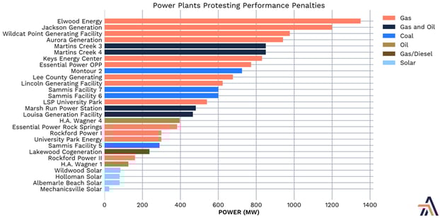
Bar graphs are probably the most widely used and most easily understood variety. We usually use bar graphs to show some value that is representative of a discrete entity or category. In PJM Performance During Winter Storm Elliot Shows Many Flaws, we used the following bar graph to show the size of different power plants that were protesting performance penalties following Winter Storm Elliot. To add another data dimension, color was employed to indicate the type of fuel used by the individual plants.

Demonstrating Relationships with Scatter Plots

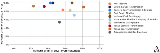
Scatter plots can be used to demonstrate the relationship between two variables for individual entities. In EPA Proposes Applying Good Neighbor Rule to Certain Compressor Stations, the above graph is used to visually identify the relationship between the percent of horsepower that is located in states subject to the EPA’s good neighbor regulations versus the percent of horsepower that exists in compressor stations with less than 5,000 horsepower for those pipelines. In this example, there is not a strong relationship between the two variables.

It is not uncommon, however, to identify a stronger correlation between variables using a scatter plot. That correlation can either be positive (where higher values of one variable often indicate higher values of the other variable) or negative (where a higher value of one variable typically results in a lower value of the other).

Showing Changes Over Time with Line Graphs

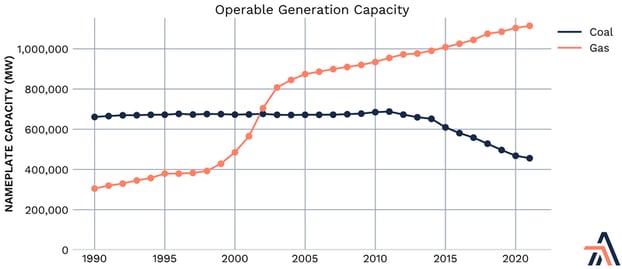
In Biden White House Tries to Force FERC’s Hand on GHGs, we used the line graph below to show the change in operable generation capacity fired by coal and natural gas from 1990 through today. Line graphs are frequently used to demonstrate the change in a specific value over time. Like the bar graph above, we again used color to differentiate between fuel types to provide another layer of information.

Putting Together the Pieces with Area Graphs

Area graphs are similar to line graphs in that they show how a certain value changes over time. However, it isn’t uncommon for this type of graph to be misinterpreted. The individual areas are not meant to be read as individual values, but rather as a piece of the whole. When we use area graphs, we stack these pieces to show how things build up and work together as part of the bigger picture.

A line graph can be layered on top of an area graph. In Coal to Gas: Energy Evolution Stage One, we used this technique to show not only the change in share of electric generation in the United States over time, but also how emissions from the electric power sector have changed in the same time period.

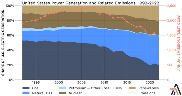
Because we use the percent share of generation in the above graph, it is clear that this graph represents how the different generation sources add together to account for total electricity production. While coal and natural gas have together accounted for about 65% of annual generation since 1990, natural gas has steadily grown to account for the majority of that piece of generation. An incorrect interpretation of this graph would be to say that, in 1990, natural gas accounted for 65% of the total generation. By adding in the line for emissions, we can show that, as natural gas generation has increased and taken the place of coal-fired generation, emissions have fallen in that same time period.

Displaying Distributions with Box Plots and Swarm Plots

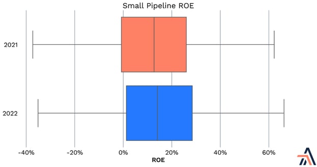
In Gas Pipelines See Some Uplift in Returns for 2022 as Compared to 2021, we utilize both a box plot and a swarm plot to show the distribution of ROEs for different pipelines in 2021 and 2022.

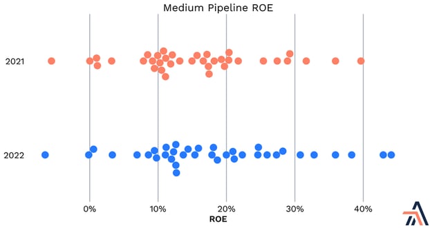
The swarm plot above has a dot for the ROE of each pipeline in both 2021 and 2022. The box plot below shows a similar set of data, but as an aggregation rather than individual points. The lines on either side of the box are often referred to as whiskers, so you’ll see this type of graph also referred to as a “box-and-whisker” plot. In this example, the box itself goes from the 25th percentile to the 75th percentile, and the line within the box is representative of the median. The whisker on the left-hand side goes from the lowest ROE to the 25th percentile and the line on the right-hand side of the box goes from the 75th percentile to the largest ROE. The 25th and 75th percentiles are often referred to as the first and third quartiles, respectively. In some cases, there will be extra dots on one or both sides of the whiskers, and these points are considered statistical outliers.

Illustrating Key Milestones with Timelines

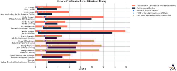
The Arbo team routinely looks at project timing and key milestones. In A Tale of Two Chairmen: Presidents’ Day Presidential Permitting, we created the following timeline visual to show the length of time it has taken for past projects not only to receive their Presidential Permits, but also the length of environmental review and when other key milestones occurred as part of that process. Looking at this data in a visual format provides a strong sense of how long this process usually takes, and makes it easier to compare multiple project timelines.

Bringing in Geographic Elements with Maps

One of our favorite ways to visualize information is by putting it on a map. In Acting Chairman Phillips Appears to Be Enforcing Key Aspects of the Failed Draft Certificate Policy Statement, the following map is used to show the locations of different environmental justice communities in Alabama, with the color of the community indicating the reason for its designation.

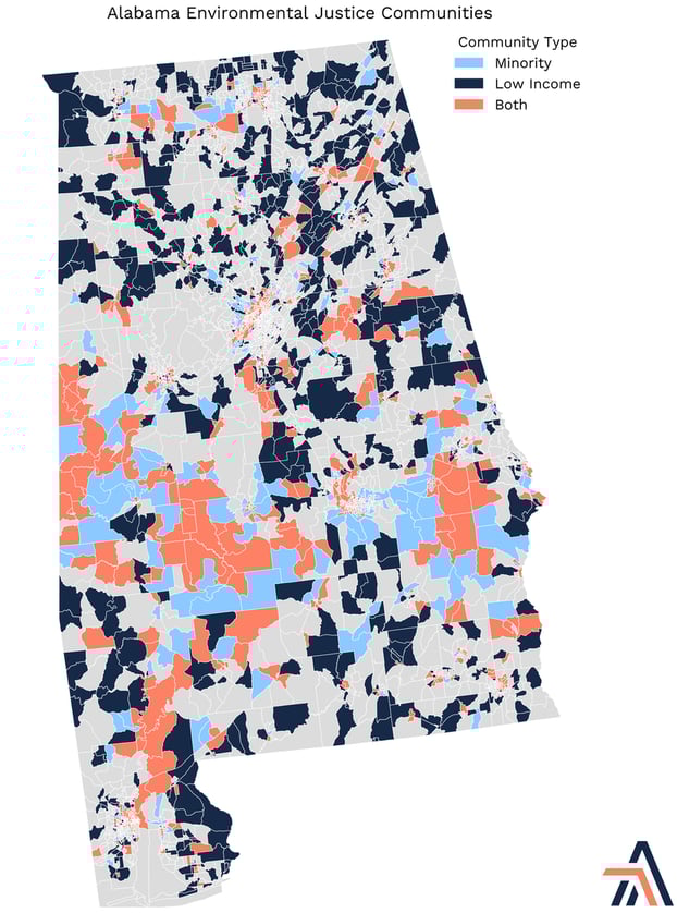
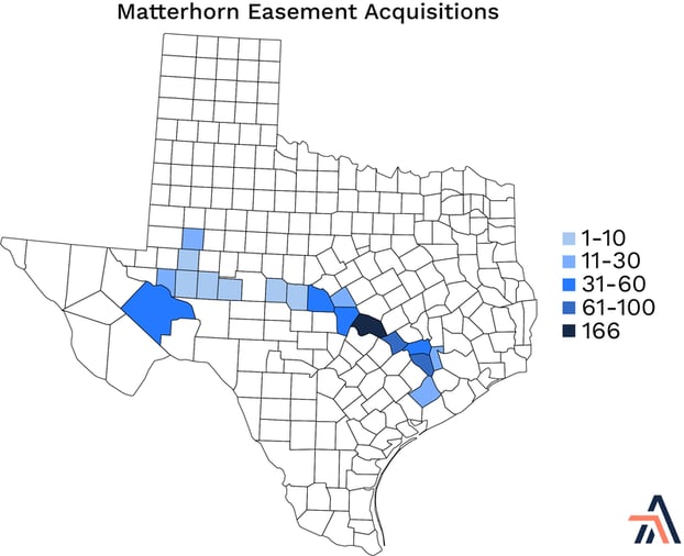
In the case of the preceding map, we displayed the communities by census block, but more often, we look at relevant data at the county- or state-level. For example, the map below from Permian Gas Takeaway Looks to Grow This Year and Next shows the number of easements Matterhorn has acquired in Texas counties along its route.

On a request basis, we also map individual pipeline footprints and their proximity to other sites, such as solar generation facilities or landfills, that may provide renewable natural gas opportunities.